4.14.5.35.1.12. LiquefiedSand
- hystereticBackbone('LiquefiedSand', backboneTag, X, D, kN, m)
- The p-y curve model of liquefied sand is recommended
in Rollins (2005) based on the full-scale lateral load tests to analyze the laterally loaded single piles when the liquefied sand layer is present.
The backbone function is defined in manual
backboneTag(int)integer tag identifying the backbone function.
X(float)the depth.
D(float)is the pile diameter
kN(float)Since the model assumes the metric units, if your units are different to, define kN to match your unit system.
m(float)Define the unit meter for the same reason of kN
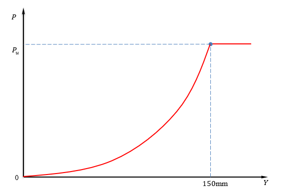
The typical p-y curve for liquefied sand is shown in the figure above. The pile lateral soil resistance, P, increases with the pile deflection along a concave upward curve until the deflection reaches 150 mm. Note that \(P_u\) is the ultimate lateral resistance when the pile deflection (y value) is equal to or greater than 150 mm.
The following equations are proposed by Rollins et al. (2005) to estimate the mobilization of pile lateral soil resistance (P) with deflection (y):
Note that A, B, and C in the equations above are the curve fitting parameters that depend on the depth (X). D is the pile diameter. \(P_d\) is the pile diameter correction factor and it is limited to the pile diameter between 0.3 m and 2.6 m.