14.2.3. Example name spaced nonlinear SDOF
The source code is developed by Maxim Millen from University of Porto.
The source code is shown below, which can be downloaded
here.Also download the
ground motion fileMake sure the numpy, matplotlib and eqsig packages are installed in your Python distribution.
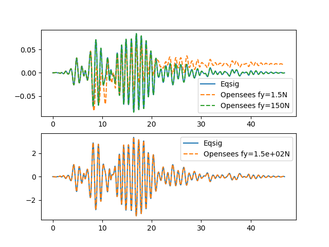
Run the source code in your favorite Python program and should see
  1import requests
  2import eqsig
  3import matplotlib.pyplot as plt
  4import numpy as np
  5from os.path import exists
  6
  7import openseespy.opensees as op
  8
  9
 10### Generating Constants #############
 11class opensees_constants:
 12    def __init__(self):
 13        self.FREE = 0
 14        self.FIXED = 1
 15
 16        self.X = 1
 17        self.Y = 2
 18        self.ROTZ = 3
 19
 20opc = opensees_constants()
 21
 22
 23def get_inelastic_response(mass, k_spring, f_yield, motion, dt, xi=0.05, r_post=0.0):
 24    """
 25    Run seismic analysis of a nonlinear SDOF
 26
 27    :param mass: SDOF mass
 28    :param k_spring: spring stiffness
 29    :param f_yield: yield strength
 30    :param motion: list, acceleration values
 31    :param dt: float, time step of acceleration values
 32    :param xi: damping ratio
 33    :param r_post: post-yield stiffness
 34    :return:
 35    """
 36
 37    op.wipe()
 38    op.model('basic', '-ndm', 2, '-ndf', 3)  # 2 dimensions, 3 dof per node
 39
 40    # Establish nodes
 41    bot_node = 1
 42    top_node = 2
 43    op.node(bot_node, 0., 0.)
 44    op.node(top_node, 0., 0.)
 45
 46    # Fix bottom node
 47    op.fix(top_node, opc.FREE, opc.FIXED, opc.FIXED)
 48    op.fix(bot_node, opc.FIXED, opc.FIXED, opc.FIXED)
 49    # Set out-of-plane DOFs to be slaved
 50    op.equalDOF(1, 2, *[2, 3])
 51
 52    # nodal mass (weight / g):
 53    op.mass(top_node, mass, 0., 0.)
 54
 55    # Define material
 56    bilinear_mat_tag = 1
 57    mat_type = "Steel01"
 58    mat_props = [f_yield, k_spring, r_post]
 59    op.uniaxialMaterial(mat_type, bilinear_mat_tag, *mat_props)
 60
 61    # Assign zero length element
 62    beam_tag = 1
 63    op.element('zeroLength', beam_tag, bot_node, top_node, "-mat", bilinear_mat_tag, "-dir", 1, '-doRayleigh', 1)
 64
 65    # Define the dynamic analysis
 66    load_tag_dynamic = 1
 67    pattern_tag_dynamic = 1
 68
 69    values = list(-1 * motion)  # should be negative
 70    op.timeSeries('Path', load_tag_dynamic, '-dt', dt, '-values', *values)
 71    op.pattern('UniformExcitation', pattern_tag_dynamic, opc.X, '-accel', load_tag_dynamic)
 72
 73    # set damping based on first eigen mode
 74    eigen_1 = op.eigen('-fullGenLapack', 1)
 75    angular_freq = eigen_1[0] ** 0.5
 76    alpha_m = 0.0
 77    beta_k = 2 * xi / angular_freq
 78    beta_k_comm = 0.0
 79    beta_k_init = 0.0
 80
 81    op.rayleigh(alpha_m, beta_k, beta_k_init, beta_k_comm)
 82
 83    # Run the dynamic analysis
 84
 85    op.wipeAnalysis()
 86
 87    op.algorithm('Newton')
 88    op.system('SparseGeneral')
 89    op.numberer('RCM')
 90    op.constraints('Transformation')
 91    op.integrator('Newmark', 0.5, 0.25)
 92    op.analysis('Transient')
 93
 94    tol = 1.0e-10
 95    iterations = 10
 96    op.test('EnergyIncr', tol, iterations, 0, 2)
 97    analysis_time = (len(values) - 1) * dt
 98    analysis_dt = 0.001
 99    outputs = {
100        "time": [],
101        "rel_disp": [],
102        "rel_accel": [],
103        "rel_vel": [],
104        "force": []
105    }
106
107    while op.getTime() < analysis_time:
108        curr_time = op.getTime()
109        op.analyze(1, analysis_dt)
110        outputs["time"].append(curr_time)
111        outputs["rel_disp"].append(op.nodeDisp(top_node, 1))
112        outputs["rel_vel"].append(op.nodeVel(top_node, 1))
113        outputs["rel_accel"].append(op.nodeAccel(top_node, 1))
114        op.reactions()
115        outputs["force"].append(-op.nodeReaction(bot_node, 1))  # Negative since diff node
116    op.wipe()
117    for item in outputs:
118        outputs[item] = np.array(outputs[item])
119
120    return outputs
121
122
123def show_single_comparison(acc_signal):
124    """
125    Create a plot of an elastic analysis, nonlinear analysis and closed form elastic
126
127    :param acc_signal: input acceleration ground motion (as eqsig.AccSignal)
128
129    :return:
130    """
131
132    rec = acc_signal.values
133    motion_step = acc_signal.dt
134
135    period = 1.0
136    xi = 0.05
137    mass = 1.0
138    f_yield = 1.5  # Reduce this to make it nonlinear
139    r_post = 0.0
140
141    periods = np.array([period])
142    resp_u, resp_v, resp_a = eqsig.sdof.response_series(motion=rec, dt=motion_step, periods=periods, xi=xi)
143
144    k_spring = 4 * np.pi ** 2 * mass / period ** 2
145    outputs = get_inelastic_response(mass, k_spring, f_yield, motion=rec, dt=motion_step, xi=xi, r_post=r_post)
146    outputs_elastic = get_inelastic_response(mass, k_spring, f_yield * 100, rec,
147                                             motion_step, xi=xi, r_post=r_post)
148    ux_opensees = outputs["rel_disp"]
149    ux_opensees_elastic = outputs_elastic["rel_disp"]
150
151    bf, sps = plt.subplots(nrows=2, figsize=(10,7.5))
152    sps[0].plot(acc_signal.time, resp_u[0], label="Eqsig")
153    sps[0].plot(outputs["time"], ux_opensees, label=f"Opensees fy={f_yield:.3g}N", ls="--")
154    sps[0].plot(outputs["time"], ux_opensees_elastic, label=f"Opensees fy={(f_yield * 100):.3g}N", ls="--")
155    sps[1].plot(acc_signal.time, resp_a[0], label="Eqsig")  # Elastic solution
156    time = acc_signal.time
157    acc_opensees_elastic = np.interp(time, outputs_elastic["time"], outputs_elastic["rel_accel"]) - rec
158    print("diff", sum(acc_opensees_elastic - resp_a[0]))
159    sps[1].plot(time, acc_opensees_elastic, label=f"Opensees fy={(f_yield * 100):.2g}N", ls="--")
160    sps[0].set_xlim(xmin=0, xmax=None)
161    sps[0].legend()
162    sps[1].set_xlim(xmin=0, xmax=None)
163    sps[1].legend()
164    for sp in sps:
165        sp.legend()
166        sp.set_xlabel('Time (s)')
167        sp.grid(True)
168    sps[0].set_ylabel('Displacements (m)')
169    sps[1].set_ylabel('Accelerations (m/s^2)')
170    plt.show()
171
172
173if __name__ == '__main__':
174    ### Importing Ground Motion #############
175    if exists('test_motion_dt0p01.txt'):
176        with open('test_motion_dt0p01.txt','r') as filestream:
177            eq_motion = [float(item.strip()) for item in filestream if item.strip() != '']
178    else:
179        eq_url = r'https://openseespydoc.readthedocs.io/en/latest/_downloads/92ed0c80b09bea0d28bf940a5dc4c3f4/test_motion_dt0p01.txt'
180        response = requests.get(eq_url)
181        # response.encoding = "utf-8" # utf-8 or iso8859-1
182        #eq_motion = response.text.split('\n')
183        eq_motion = [float(item.strip()) for item in response.text.split('\n') if item.strip() != '']
184
185    eq_motion_dt = 0.01
186
187    acc_signal = eqsig.AccSignal(eq_motion, eq_motion_dt)
188
189    ### Running Analysis #############
190    show_single_comparison(acc_signal)