14.2.2. Reinforced Concrete Frame Earthquake Analysis

1. The source code is shown below, which can be downloaded here.

2. The file for gravity analysis is also needed here.

3. The ReadRecord is a useful python function for parsing the PEER strong motion data base files and returning the dt, nPts and creating a file containing just data points. The function is kept in a seperate file here and is imported in the example.

4. The ground motion data file here must be put in the same folder.

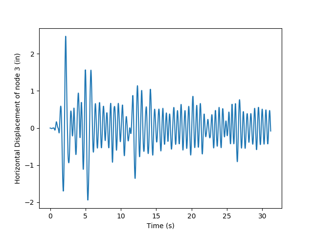
5. Run the source code in your favorite Python program and should see Passed! in the results and a plotting of displacement for node 3

print("==========================")
print("Start RCFrameEarthquake Example")

# Units: kips, in, sec  
#
# Written: Minjie

from openseespy.opensees import *

import ReadRecord
import numpy as np
import matplotlib.pyplot as plt

wipe()
# ----------------------------------------------------
# Start of Model Generation & Initial Gravity Analysis
# ----------------------------------------------------

# Do operations of Example3.1 by sourcing in the tcl file
import RCFrameGravity
print("Gravity Analysis Completed")

# Set the gravity loads to be constant & reset the time in the domain
loadConst('-time', 0.0)

# ----------------------------------------------------
# End of Model Generation & Initial Gravity Analysis
# ----------------------------------------------------

# Define nodal mass in terms of axial load on columns
g = 386.4
m = RCFrameGravity.P/g

mass(3, m, m, 0.0)
mass(4, m, m, 0.0)

# Set some parameters
record = 'elCentro'

# Permform the conversion from SMD record to OpenSees record
dt, nPts = ReadRecord.ReadRecord(record+'.at2', record+'.dat')

# Set time series to be passed to uniform excitation
timeSeries('Path', 2, '-filePath', record+'.dat', '-dt', dt, '-factor', g)

# Create UniformExcitation load pattern
#                         tag dir 
pattern('UniformExcitation',  2,   1,  '-accel', 2)

# set the rayleigh damping factors for nodes & elements
rayleigh(0.0, 0.0, 0.0, 0.000625)

# Delete the old analysis and all it's component objects
wipeAnalysis()

# Create the system of equation, a banded general storage scheme
system('BandGeneral')

# Create the constraint handler, a plain handler as homogeneous boundary
constraints('Plain')

# Create the convergence test, the norm of the residual with a tolerance of 
# 1e-12 and a max number of iterations of 10
test('NormDispIncr', 1.0e-12,  10 )

# Create the solution algorithm, a Newton-Raphson algorithm
algorithm('Newton')

# Create the DOF numberer, the reverse Cuthill-McKee algorithm
numberer('RCM')

# Create the integration scheme, the Newmark with alpha =0.5 and beta =.25
integrator('Newmark',  0.5,  0.25 )

# Create the analysis object
analysis('Transient')

# Perform an eigenvalue analysis
numEigen = 2
eigenValues = eigen(numEigen)
print("eigen values at start of transient:",eigenValues)

# set some variables
tFinal = nPts*dt
tCurrent = getTime()
ok = 0

time = [tCurrent]
u3 = [0.0]

# Perform the transient analysis
while ok == 0 and tCurrent < tFinal:
    
    ok = analyze(1, .01)
    
    # if the analysis fails try initial tangent iteration
    if ok != 0:
        print("regular newton failed .. lets try an initail stiffness for this step")
        test('NormDispIncr', 1.0e-12,  100, 0)
        algorithm('ModifiedNewton', '-initial')
        ok =analyze( 1, .01)
        if ok == 0:
            print("that worked .. back to regular newton")
        test('NormDispIncr', 1.0e-12,  10 )
        algorithm('Newton')
    
    tCurrent = getTime()

    time.append(tCurrent)
    u3.append(nodeDisp(3,1))



# Perform an eigenvalue analysis
eigenValues = eigen(numEigen)
print("eigen values at end of transient:",eigenValues)

results = open('results.out','a+')

if ok == 0:
    results.write('PASSED : RCFrameEarthquake.py\n');
    print("Passed!")
else:
    results.write('FAILED : RCFrameEarthquake.py\n');
    print("Failed!")

results.close()

plt.plot(time, u3)
plt.ylabel('Horizontal Displacement of node 3 (in)')
plt.xlabel('Time (s)')

plt.show()



print("==========================")