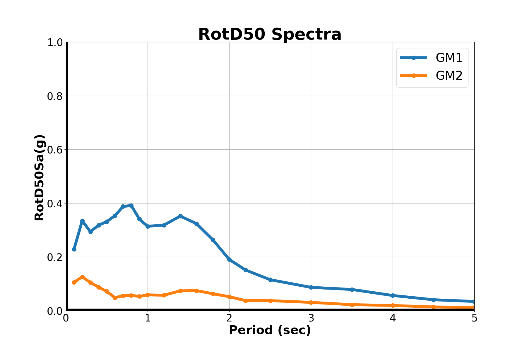
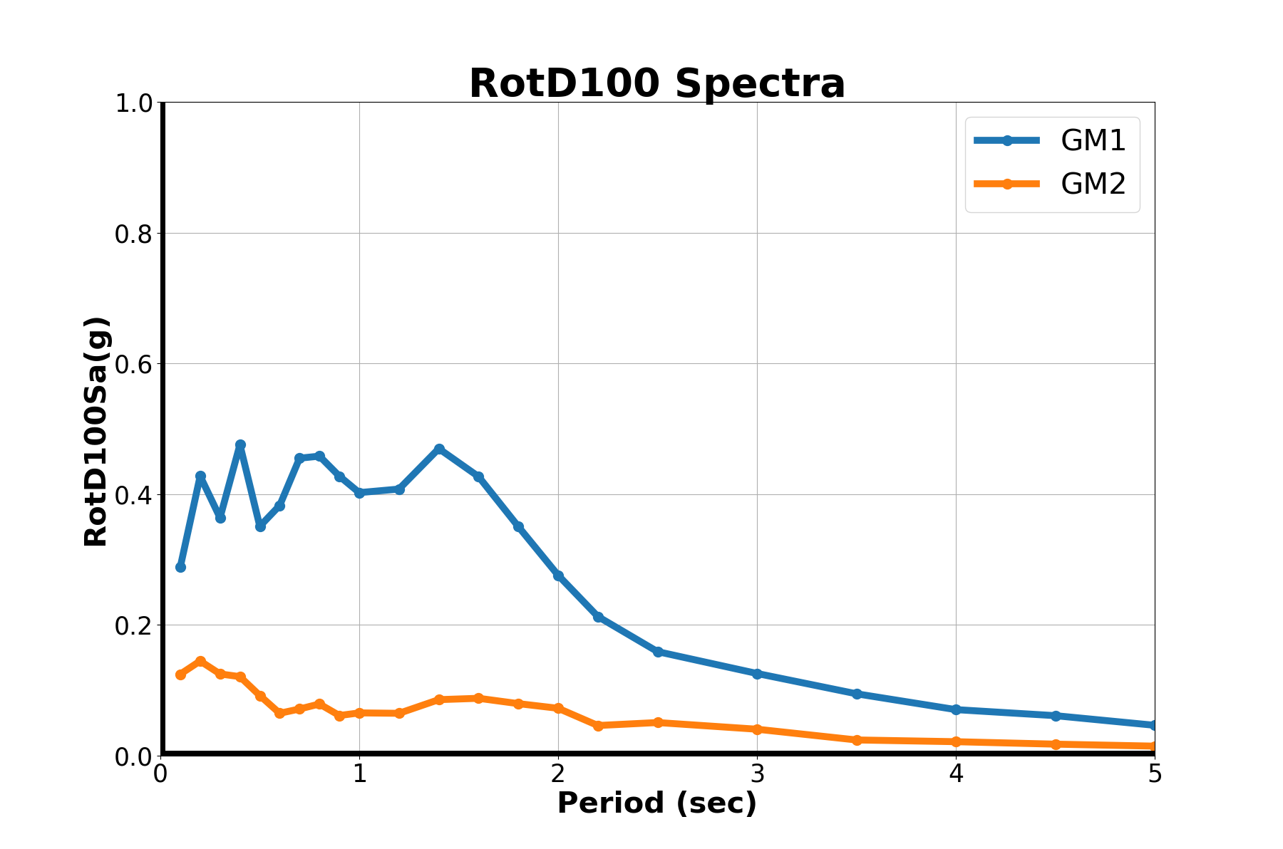
14.2.4. RotD Spectra of Ground Motion
The source code is developed by Jawad Fayaz from University of California- Irvine.
The source code is shown below, which can be downloaded
here.Also download the code to read the provided GM file
here.The example bi-directional ground motion time histories are given
GM11,GM21,GM12,GM22.Run the source code in any Python IDE (e.g Spyder, Jupyter Notebook) and should see
"""
author : JAWAD FAYAZ (email: jfayaz@uci.edu) (website: https://jfayaz.github.io)

------------------------------ Instructions -------------------------------------
This code develops the RotD50 Sa and RotD100 Sa Spectra of the Bi-Directional
Ground Motion records as '.AT2' files provided in the current directory

The two directions of the ground motion record must be named as 'GM1i' and 'GM2i',
where 'i' is the ground motion number which goes from 1 to 'n', 'n' being the total
number of ground motions for which the Spectra needs to be generated. The extension
of the files must be '.AT2'

For example: If the Spectra of two ground motion records are required, 4 files with
the following names must be provided in the given 'GM' folder:
    'GM11.AT2' - Ground Motion 1 in direction 1 (direction 1 can be either one of the bi-directional GM as we are rotating the ground motions it does not matter)
    'GM21.AT2' - Ground Motion 1 in direction 2 (direction 2 is the other direction of the bi-directional GM)
    'GM12.AT2' - Ground Motion 2 in direction 1 (direction 1 can be either one of the bi-directional GM as we are rotating the ground motions it does not matter)
    'GM22.AT2' - Ground Motion 2 in direction 2 (direction 2 is the other direction of the bi-directional GM)

The Ground Motion file must be a vector file with 4 header lines.The first 3 lines can have
any content, however, the 4th header line must be written exactly as per the following example:
    'NPTS=  15864, DT= 0.0050'
The 'ReadGMFile.py' can be edited accordingly  for any other format

You may run this code in python IDE: 'Spyder' or any other similar IDE

Make sure you have the following python libraries installed:
    os
    sys
    pathlib
    fnmatch
    shutil
    IPython
    pandas
    numpy
    matplotlib.pyplot

INPUT:
This codes provides the option to have 3 different regions of developing the Spectra of ground motions with different period intervals (discretizations)
The following inputs within the code are required:
    'Path_to_openpyfiles'--> Path where the library files 'opensees.pyd' and 'LICENSE.rst' of OpenSeesPy are included (for further details go to https://openseespydoc.readthedocs.io/en/latest/windows.html)
    'Int_T_Reg_1'        --> Period Interval for the first region of the Spectrum
    'End_T_Reg_1'        --> Last Period of the first region of the Spectrum (where to end the first region)
    'Int_T_Reg_2'        --> Period Interval for the second region of the Spectrum
    'End_T_Reg_2'        --> Last Period of the second region of the Spectrum (where to end the second region)
    'Int_T_Reg_3'        --> Period Interval for the third region of the Spectrum
    'End_T_Reg_3'        --> Last Period of the third region of the Spectrum (where to end the third region)
    'Plot_Spectra'       --> whether to plot the generated Spectra of the ground motions (options: 'Yes', 'No')

OUTPUT:
The output will be provided in a saperate 'GMi_Spectra.txt' file for each ground motion record, where 'i' denotes the number of ground motion in the same of
provided 'GM1i.AT2' and 'GM2i.AT2' files. The output files will be generated in a saperate folder 'Spectra' which will be created in the current folder
The 'GMi_Spectra.txt' file will consist of space-saperated file with:
    'Periods (secs)' 'RotD50 Sa (g)' 'RotD100 Sa (g)'

%%%%% ========================================================================================================================================================================= %%%%%%
%%%%%%%%%%%%%%%%%%%%%%%%%%%%%%%%%%%%%%%%%%%%%%%%%%%%%%%%%%%%%%%%%%%%%%%%%%%%%%%%%%%%%%%%%%%%%%%%%%%%%%%%%%%%%%%%%%%%%%%%%%%%%%%%%%%%%%%%%%%%%%%%%%%%%%%%%%%%%%%%%%%%%%%%%%%%%%%%%%%%%%

"""

##### ================== INPUTS  ================== #####

# Path where the library files 'opensees.pyd' and 'LICENSE.rst' are included (for further details go to https://openseespydoc.readthedocs.io/en/latest/windows.html)
Path_to_openpyfiles = 'C:\Tcl'

# For periods 0 to 'End_T_Reg_1' in an interval of 'Int_T_Reg_1'
Int_T_Reg_1       = 0.1
End_T_Reg_1       = 1

# For periods ['End_T_Reg_1'+'Int_T_Reg_2'] to 'End_T_Reg_2' in an interval of 'Int_T_Reg_2'
Int_T_Reg_2       = 0.2
End_T_Reg_2       = 2

# For periods ['End_T_Reg_2'+'Int_T_Reg_3'] to 'End_T_Reg_3' in an interval of 'Int_T_Reg_3'
Int_T_Reg_3       = 0.5
End_T_Reg_3       = 5

# Plot Spectra  (options: 'Yes' or 'No')
Plot_Spectra      = 'Yes'


##### =============== CODE BEGINS ================ #######
## Importing Libraries
import os, sys, pathlib, fnmatch
import shutil as st
from IPython import get_ipython

from openseespy.opensees import *

import pandas as pd
import numpy as np
import matplotlib.pyplot as plt
import warnings
import matplotlib.cbook
warnings.filterwarnings("ignore",category=matplotlib.cbook.mplDeprecation)
wipe()

# Getting Number of Ground Motions from the GM folder
GMdir = os.getcwd()
No_of_GMs = int(len(fnmatch.filter(os.listdir(GMdir),'*.AT2'))/2)
print('\nGenerating Spectra for {} provided GMs \n\n'.format(np.round(No_of_GMs,0)))

# Initializations
DISPLACEMENTS = pd.DataFrame(columns=['uX','uY'])
GM_SPECTRA = pd.DataFrame(columns=['Period(s)','RotD50Sa(g)', 'RotD100Sa(g)'])
SDOF_RESPONSE = [[]]
GM_RESPONSE = [[]]

# Spectra Generation
for iEQ in range(1,No_of_GMs+1):
    print('Generating Spectra for GM: {} ...\n'.format(np.round(iEQ,0)))
    Periods = np.concatenate((list(np.arange(Int_T_Reg_1,End_T_Reg_1+Int_T_Reg_1,Int_T_Reg_1)),list(np.arange(End_T_Reg_1+Int_T_Reg_2,End_T_Reg_2+Int_T_Reg_2,Int_T_Reg_2)),list(np.arange(End_T_Reg_2+Int_T_Reg_3,End_T_Reg_3+Int_T_Reg_3,Int_T_Reg_3))),axis=0)
    ii = 0

    for T in Periods:
        ii = ii+1
        GMinter = 0

        # Storing Periods
        GM_SPECTRA.loc[ii-1,'Period(s)'] = T

        # Setting modelbuilder
        model('basic', '-ndm', 3, '-ndf', 6)

        # Setting SODF Variables
        g = 386.1                   # value of g
        L = 1.0                     # Length
        d = 2                       # Diameter
        r = d/2                     # Radius
        A = np.pi*(r**2)            # Area
        E = 1.0                     # Elastic Modulus
        G = 1.0                     # Shear Modulus
        I3 = np.pi*(r**4)/4         # Moment of Inertia (zz)
        J = np.pi*(r**4)/2          # Polar Moment of Inertia
        I2 = np.pi*(r**4)/4         # Moment of Inertia (yy)
        K = 3*E*I3/(L**3)           # Stiffness
        M = K*(T**2)/4/(np.pi**2)   # Mass
        omega = np.sqrt(K/M)        # Natural Frequency
        Tn = 2*np.pi/omega          # Natural Period

        # Creating nodes
        node(1, 0.0, 0.0, 0.0)
        node(2, 0.0, 0.0, L)

        # Transformation
        transfTag = 1
        geomTransf('Linear',transfTag,0.0,1.0,0.0)

        # Setting boundary condition
        fix(1, 1, 1, 1, 1, 1, 1)

        # Defining materials
        uniaxialMaterial("Elastic", 11, E)

        # Defining elements
        element("elasticBeamColumn",12,1,2,A,E,G,J,I2,I3,1)

        # Defining mass
        mass(2,M,M,0.0,0.0,0.0,0.0)

        # Eigen Value Analysis (Verifying Period)
        numEigen = 1
        eigenValues = eigen(numEigen)
        omega = np.sqrt(eigenValues)
        T = 2*np.pi/omega
        print('   Calculating Spectral Ordinate for Period = {} secs'.format(np.round(T,3)))

        ## Reading GM Files
        exec(open("ReadGMFile.py").read())	            # read in procedure Multinition
        iGMinput = 'GM1'+str(iEQ)+' GM2'+str(iEQ) ;
        GMinput  = iGMinput.split(' ');
        gmXY     = {}
        for i in range(0,2):
            inFile   = GMdir + '\\'+ GMinput[i]+'.AT2';
            dt, NumPts , gmXY = ReadGMFile()

        # Storing GM Histories
        gmX = gmXY[1]
        gmY = gmXY[2]
        gmXY_mat = np.column_stack((gmX,gmX,gmY,gmY))

        # Bidirectional Uniform Earthquake ground motion (uniform acceleration input at all support nodes)
        iGMfile      = 'GM1'+str(iEQ)+' GM2'+str(iEQ) ;
        GMfile       = iGMfile.split(' ')
        GMdirection  = [1,1,2,2];
        GMfact	     = [np.cos(GMinter*np.pi/180),np.sin(-GMinter*np.pi/180), np.sin(GMinter*np.pi/180), np.cos(GMinter*np.pi/180)];
        IDTag        = 2
        loop         = [1,2,3,4]

        for i in loop:
            # Setting time series to be passed to uniform excitation
            timeSeries('Path',IDTag +i, '-dt', dt, '-values', *list(gmXY_mat[:,i-1]), '-factor', GMfact[i-1]*g)
            # Creating UniformExcitation load pattern
            pattern('UniformExcitation',  IDTag+i,   GMdirection[i-1],  '-accel', IDTag+i)

        # Defining Damping
        # Applying Rayleigh Damping from $xDamp
        # D=$alphaM*M + $betaKcurr*Kcurrent + $betaKcomm*KlastCommit + $beatKinit*$Kinitial
        xDamp 		= 0.05;								# 5% damping ratio
        alphaM 		= 0.;								# M-prop. damping; D = alphaM*M
        betaKcurr 	= 0.;         						# K-proportional damping;      +beatKcurr*KCurrent
        betaKcomm 	= 2.*xDamp/omega;   				# K-prop. damping parameter;   +betaKcomm*KlastCommitt
        betaKinit 	= 0.;         						# initial-stiffness proportional damping      +beatKinit*Kini
        rayleigh(alphaM,betaKcurr,betaKinit,betaKcomm); # RAYLEIGH damping

        # Creating the analysis
        wipeAnalysis()			            # clear previously-define analysis parameters
        constraints("Penalty",1e18, 1e18)   # how to handle boundary conditions
        numberer("RCM")                     # renumber dof's to minimize band-width (optimization), if you want to
        system('SparseGeneral')             # how to store and solve the system of equations in the analysis
        algorithm('Linear')	                # use Linear algorithm for linear analysis
        integrator("TRBDF2")                # determine the next time step for an analysis
        algorithm("NewtonLineSearch")       # define type of analysis: time-dependent
        test('EnergyIncr',1.0e-6, 100, 0)
        analysis("Transient")

        # Variables (Can alter the speed of analysis)
        dtAnalysis    = dt
        TmaxAnanlysis = dt*NumPts
        tFinal        = int(TmaxAnanlysis/dtAnalysis)
        tCurrent      = getTime()
        ok            = 0
        time          = [tCurrent]

        # Initializations of response
        u1            = [0.0]
        u2            = [0.0]

        # Performing the transient analysis (Performance is slow in this loop, can be altered by changing the parameters)
        while ok == 0 and tCurrent < tFinal:
            ok = analyze(1, dtAnalysis)
            # if the analysis fails try initial tangent iteration
            if ok != 0:
                print("Iteration failed .. lets try an initial stiffness for this step")
                test('NormDispIncr', 1.0e-12,  100, 0)
                algorithm('ModifiedNewton', '-initial')
                ok =analyze( 1, .001)

                if ok == 0:
                    print("that worked .. back to regular newton")
                    test('NormDispIncr', 1.0e-12,  10 )
                    algorithm('Newton')

            tCurrent = getTime()
            time.append(tCurrent)
            u1.append(nodeDisp(2,1))
            u2.append(nodeDisp(2,2))

        # Storing responses
        DISPLACEMENTS.loc[ii-1,'uX'] = np.array(u1)
        DISPLACEMENTS.loc[ii-1,'uY'] = np.array(u2)
        DISP_X_Y = np.column_stack((np.array(u1),np.array(u2)))

        # Rotating the Spectra (Projections)
        Rot_Matrix = np.zeros((2,2))
        Rot_Disp = np.zeros((180,1))
        for theta in range (0,180,1):
            Rot_Matrix [0,0] = np.cos(np.deg2rad(theta))
            Rot_Matrix [0,1] = np.sin(np.deg2rad(-theta))
            Rot_Matrix [1,0] = np.sin(np.deg2rad(theta))
            Rot_Matrix [1,1] = np.cos(np.deg2rad(theta))
            Rot_Disp[theta,0] = np.max(np.matmul(DISP_X_Y,Rot_Matrix)[:,0])

        # Storing Spectra
        Rot_Acc = np.dot(Rot_Disp,(omega**2)/g)
        GM_SPECTRA.loc[ii-1,'RotD50Sa(g)'] = np.median(Rot_Acc)
        GM_SPECTRA.loc[ii-1,'RotD100Sa(g)']= np.max(Rot_Acc)
        wipe()

    # Writing Spectra to Files
    if not os.path.exists('Spectra'):
        os.makedirs('Spectra')
    GM_SPECTRA.to_csv('Spectra//GM'+str(iEQ)+'_Spectra.txt', sep=' ',header=True,index=False)

    # Plotting Spectra
    if Plot_Spectra == 'Yes':

        def plot_spectra(PlotTitle,SpectraType,iGM):
            axes = fig.add_subplot(1, 1, 1)
            axes.plot(GM_SPECTRA['Period(s)'] , GM_SPECTRA[SpectraType] , '.-',lw=7,markersize=20, label='GM'+str(iGM))
            axes.set_xlabel('Period (sec)',fontsize=30,fontweight='bold')
            axes.set_ylabel(SpectraType,fontsize=30,fontweight='bold')
            axes.set_title(PlotTitle,fontsize=40,fontweight='bold')
            axes.tick_params(labelsize= 25)
            axes.grid(True)
            axes.set_xlim(0, np.ceil(max(GM_SPECTRA['Period(s)'])))
            axes.set_ylim(0, np.ceil(max(GM_SPECTRA[SpectraType])))
            axes.axhline(linewidth=10,color='black')
            axes.axvline(linewidth=10,color='black')
            axes.hold(True)
            axes.legend(fontsize =30)

        fig = plt.figure(1,figsize=(18,12))
        plot_spectra('RotD50 Spectra','RotD50Sa(g)',iEQ)

        fig = plt.figure(2,figsize=(18,12))
        plot_spectra('RotD100 Spectra','RotD100Sa(g)',iEQ)

    SDOF_RESPONSE.insert(iEQ-1,DISPLACEMENTS)
    GM_RESPONSE.insert(iEQ-1,GM_SPECTRA)

    print('\nGenerated Spectra for GM: {}\n\n'.format(np.round(iEQ,0)))