from openseespy.opensees import *
import numpy as np
import matplotlib.pyplot as plt
# ------------------------------
# Start of model generation
# -----------------------------
# set modelbuilder
wipe()
model('basic', '-ndm', 2, '-ndf', 2)
# variables
A = 4.0
E = 29000.0
alpha = 0.05
sY = 36.0
udisp = 2.5
Nsteps = 1000
Px = 160.0
Py = 0.0
# create nodes
node(1, 0.0, 0.0)
node(2, 72.0, 0.0)
node(3, 168.0, 0.0)
node(4, 48.0, 144.0)
# set boundary condition
fix(1, 1, 1)
fix(2, 1, 1)
fix(3, 1, 1)
# define materials
uniaxialMaterial("Hardening", 1, E, sY, 0.0, alpha/(1-alpha)*E)
# define elements
element("Truss",1,1,4,A,1)
element("Truss",2,2,4,A,1)
element("Truss",3,3,4,A,1)
# create TimeSeries
timeSeries("Linear", 1)
# create a plain load pattern
pattern("Plain", 1, 1)
# Create the nodal load
load(4, Px, Py)
# ------------------------------
# Start of analysis generation
# ------------------------------
# create SOE
system("ProfileSPD")
# create DOF number
numberer("Plain")
# create constraint handler
constraints("Plain")
# create integrator
integrator("LoadControl", 1.0/Nsteps)
# create algorithm
algorithm("Newton")
# create test
test('NormUnbalance',1e-8, 10)
# create analysis object
analysis("Static")
# ------------------------------
# Finally perform the analysis
# ------------------------------
# perform the analysis
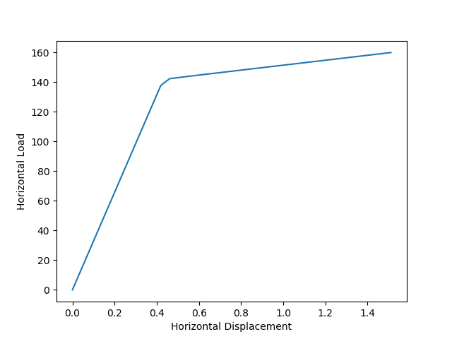
data = np.zeros((Nsteps+1,2))
for j in range(Nsteps):
analyze(1)
data[j+1,0] = nodeDisp(4,1)
data[j+1,1] = getLoadFactor(1)*Px
plt.plot(data[:,0], data[:,1])
plt.xlabel('Horizontal Displacement')
plt.ylabel('Horizontal Load')
plt.show()