from openseespy.opensees import *
import numpy as np
import matplotlib.pyplot as plt
# define model
model('basic', '-ndm', 2, '-ndf', 3)
#define node
node(1, 0.0, 0.0)
node(2, 2.0, 0.0)
node(3, 1.0, 0.0)
#define boundary condition
fix(1, 1, 1, 1)
fix(2, 1, 1, 1)
fix(3, 0, 1, 1)
#define an elastic material with Tag=1 and E=2e11.
matTag = 1
uniaxialMaterial('Steel01Thermal', 1, 2e11, 2e11, 0.01)
#define fibred section Two fibres: fiber $yLoc $zLoc $A $matTag
secTag = 1
section('FiberThermal',secTag)
fiber(-0.025, 0.0, 0.005, matTag)
fiber(0.025, 0.0, 0.005, matTag)
#define coordinate transforamtion
#three transformation types can be chosen: Linear, PDelta, Corotational)
transfTag = 1
geomTransf('Linear', transfTag)
# beam integration
np = 3
biTag = 1
beamIntegration('Lobatto',biTag, secTag, np)
#define beam element
element('dispBeamColumnThermal', 1, 1, 3, transfTag, biTag)
element('dispBeamColumnThermal', 2, 3, 2, transfTag, biTag)
# define time series
tsTag = 1
timeSeries('Linear',tsTag)
# define load pattern
patternTag = 1
maxtemp = 1000.0
pattern('Plain', patternTag, tsTag)
eleLoad('-ele', 1, '-type', '-beamThermal', 1000.0, -0.05, 1000.0, 0.05)
#eleLoad -ele 2 -type -beamThermal 0 -0.05 0 0.05
# define analysis
incrtemp = 0.01
system('BandGeneral')
constraints('Plain')
numberer('Plain')
test('NormDispIncr', 1.0e-3, 100, 1)
algorithm('Newton')
integrator('LoadControl', incrtemp)
analysis('Static')
# analysis
nstep = 100
temp = [0.0]
disp = [0.0]
for i in range(nstep):
if analyze(1) < 0:
break
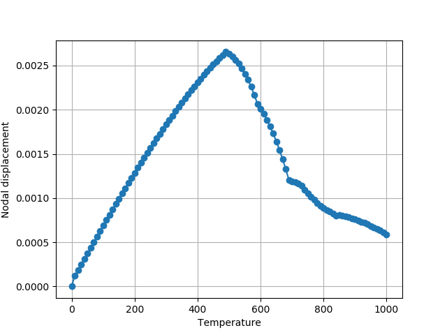
temp.append(getLoadFactor(patternTag)*maxtemp)
disp.append(nodeDisp(3,1))
plt.plot(temp,disp,'-o')
plt.xlabel('Temperature')
plt.ylabel('Nodal displacement')
plt.grid()
plt.show()