  1
  2
  3
  4
  5
  6
  7
  8
  9
 10
 11
 12
 13
 14
 15
 16
 17
 18
 19
 20
 21
 22
 23
 24
 25
 26
 27
 28
 29
 30
 31
 32
 33
 34
 35
 36
 37
 38
 39
 40
 41
 42
 43
 44
 45
 46
 47
 48
 49
 50
 51
 52
 53
 54
 55
 56
 57
 58
 59
 60
 61
 62
 63
 64
 65
 66
 67
 68
 69
 70
 71
 72
 73
 74
 75
 76
 77
 78
 79
 80
 81
 82
 83
 84
 85
 86
 87
 88
 89
 90
 91
 92
 93
 94
 95
 96
 97
 98
 99
100
101
102
103
104
105
106
107
108
109
110
111
112
113
114
115
116
117
118
119
120
121
122
123
124
125
126
127
128
129
130
131
132
133
134
135
136
137
138
139
140
141
142
143
144
145
146
147
148
149
150 | import eqsig
from eqsig import duhamels
import matplotlib.pyplot as plt
import numpy as np
import openseespy.opensees as op
import opensees_constants as opc #opensees_constants.py should be close to main file or use sys.path... to its directory
def get_inelastic_response(mass, k_spring, f_yield, motion, dt, xi=0.05, r_post=0.0):
"""
Run seismic analysis of a nonlinear SDOF
:param mass: SDOF mass
:param k_spring: spring stiffness
:param f_yield: yield strength
:param motion: list, acceleration values
:param dt: float, time step of acceleration values
:param xi: damping ratio
:param r_post: post-yield stiffness
:return:
"""
op.wipe()
op.model('basic', '-ndm', 2, '-ndf', 3) # 2 dimensions, 3 dof per node
# Establish nodes
bot_node = 1
top_node = 2
op.node(bot_node, 0., 0.)
op.node(top_node, 0., 0.)
# Fix bottom node
op.fix(top_node, opc.FREE, opc.FIXED, opc.FIXED)
op.fix(bot_node, opc.FIXED, opc.FIXED, opc.FIXED)
# Set out-of-plane DOFs to be slaved
op.equalDOF(1, 2, *[2, 3])
# nodal mass (weight / g):
op.mass(top_node, mass, 0., 0.)
# Define material
bilinear_mat_tag = 1
mat_type = "Steel01"
mat_props = [f_yield, k_spring, r_post]
op.uniaxialMaterial(mat_type, bilinear_mat_tag, *mat_props)
# Assign zero length element
beam_tag = 1
op.element('zeroLength', beam_tag, bot_node, top_node, "-mat", bilinear_mat_tag, "-dir", 1, '-doRayleigh', 1)
# Define the dynamic analysis
load_tag_dynamic = 1
pattern_tag_dynamic = 1
values = list(-1 * motion) # should be negative
op.timeSeries('Path', load_tag_dynamic, '-dt', dt, '-values', *values)
op.pattern('UniformExcitation', pattern_tag_dynamic, opc.X, '-accel', load_tag_dynamic)
# set damping based on first eigen mode
angular_freq = op.eigen('-fullGenLapack', 1) ** 0.5
alpha_m = 0.0
beta_k = 2 * xi / angular_freq
beta_k_comm = 0.0
beta_k_init = 0.0
op.rayleigh(alpha_m, beta_k, beta_k_init, beta_k_comm)
# Run the dynamic analysis
op.wipeAnalysis()
op.algorithm('Newton')
op.system('SparseGeneral')
op.numberer('RCM')
op.constraints('Transformation')
op.integrator('Newmark', 0.5, 0.25)
op.analysis('Transient')
tol = 1.0e-10
iterations = 10
op.test('EnergyIncr', tol, iterations, 0, 2)
analysis_time = (len(values) - 1) * dt
analysis_dt = 0.001
outputs = {
"time": [],
"rel_disp": [],
"rel_accel": [],
"rel_vel": [],
"force": []
}
while op.getTime() < analysis_time:
curr_time = op.getTime()
op.analyze(1, analysis_dt)
outputs["time"].append(curr_time)
outputs["rel_disp"].append(op.nodeDisp(top_node, 1))
outputs["rel_vel"].append(op.nodeVel(top_node, 1))
outputs["rel_accel"].append(op.nodeAccel(top_node, 1))
op.reactions()
outputs["force"].append(-op.nodeReaction(bot_node, 1)) # Negative since diff node
op.wipe()
for item in outputs:
outputs[item] = np.array(outputs[item])
return outputs
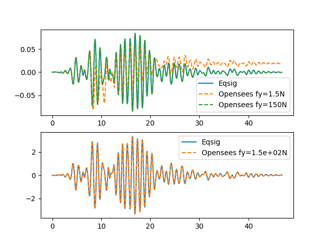
def show_single_comparison():
"""
Create a plot of an elastic analysis, nonlinear analysis and closed form elastic
:return:
"""
record_filename = 'test_motion_dt0p01.txt'
motion_step = 0.01
rec = np.loadtxt(record_filename)
acc_signal = eqsig.AccSignal(rec, motion_step)
period = 1.0
xi = 0.05
mass = 1.0
f_yield = 1.5 # Reduce this to make it nonlinear
r_post = 0.0
periods = np.array([period])
resp_u, resp_v, resp_a = duhamels.response_series(motion=rec, dt=motion_step, periods=periods, xi=xi)
k_spring = 4 * np.pi ** 2 * mass / period ** 2
outputs = get_inelastic_response(mass, k_spring, f_yield, rec, motion_step, xi=xi, r_post=r_post)
outputs_elastic = get_inelastic_response(mass, k_spring, f_yield * 100, rec, motion_step, xi=xi, r_post=r_post)
ux_opensees = outputs["rel_disp"]
ux_opensees_elastic = outputs_elastic["rel_disp"]
bf, sps = plt.subplots(nrows=2)
sps[0].plot(acc_signal.time, resp_u[0], label="Eqsig")
sps[0].plot(outputs["time"], ux_opensees, label="Opensees fy=%.3gN" % f_yield, ls="--")
sps[0].plot(outputs["time"], ux_opensees_elastic, label="Opensees fy=%.3gN" % (f_yield * 100), ls="--")
sps[1].plot(acc_signal.time, resp_a[0], label="Eqsig") # Elastic solution
time = acc_signal.time
acc_opensees_elastic = np.interp(time, outputs_elastic["time"], outputs_elastic["rel_accel"]) - rec
print("diff", sum(acc_opensees_elastic - resp_a[0]))
sps[1].plot(time, acc_opensees_elastic, label="Opensees fy=%.2gN" % (f_yield * 100), ls="--")
sps[0].legend()
sps[1].legend()
plt.show()
if __name__ == '__main__':
show_single_comparison()
|