4.14.5.35.1.10. CementedSoil
- hystereticBackbone('CementedSoil', backboneTag, pM, pU, Kpy, z, b)
The Evans and Duncan (1982) SILT model can be found here
backboneTag(int)integer tag identifying the backbone function.
pM(float)soil resistance at point M in figure below
pU(float)Evans and Duncan (1982) proposed a procedure for developing p-y curves and deciding pU, the ultimate soil resistance, in silty soils, which also defines the point U
Kpy(float)The initial modulus of subgrade reaction defines the initial straight line between O and K in figure below
z(float)the depth below ground surface to p-y curve.
b(float)diameter (width) of the pile.
There are no available recommendations on developing p-y curves for soil with cohesion and friction angle that are generally accepted. Generally, in design, the soil is classified in only two different types: cohesive or cohesionless. In the practice, this simplification leads to a significantly conservative design in the case of cemented soil or silt, which always neglects the soil resistance from the cohesion component (Juirnarongrit et al. 2005).
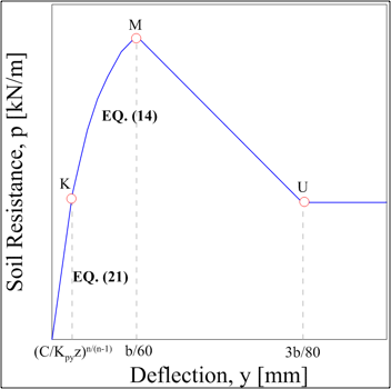
The initial straight line (EQ. 21) is defined as
the parabolic portion (EQ. 14) is defined as
where
The point \(K\) is defined at \(y_K = (C/(K_{py}z))^{n/(n-1)}\) and \(p_K = y_KK_{py}\).
The point \(M\) is defined at \(y_M = b/60\) and \(p_M\).
The point \(U\) is defined at \(y_U = 3b/80\) and \(p_U\).